kmodesFlow package
 Example table output produced from package
The kmodesFlow package provides a set of convenience functions to accompany the klaR::kmodes() function, improving overall workflow with kmodes modeling. To demo the functionality of the package, I will use a dataset on Telco customer churn (see more on the data here: https://www.kaggle.com/datasets/blastchar/telco-customer-churn).
Loading data and packages
library(kmodesFlow) # loading package
library(tidyverse)
## ── Attaching packages ─────────────────────────────────────── tidyverse 1.3.1 ──## ✔ ggplot2 3.4.0 ✔ purrr 0.3.5
## ✔ tibble 3.1.8 ✔ dplyr 1.0.10
## ✔ tidyr 1.2.0 ✔ stringr 1.4.1
## ✔ readr 2.1.2 ✔ forcats 0.5.1## ── Conflicts ────────────────────────────────────────── tidyverse_conflicts() ──
## ✖ dplyr::filter() masks stats::filter()
## ✖ dplyr::lag() masks stats::lag()data <- read_csv("telco_customer_churn.csv") # loading data as tibble## Rows: 7043 Columns: 21## ── Column specification ────────────────────────────────────────────────────────
## Delimiter: ","
## chr (17): customerID, gender, Partner, Dependents, PhoneService, MultipleLin...
## dbl (4): SeniorCitizen, tenure, MonthlyCharges, TotalCharges
##
## ℹ Use `spec()` to retrieve the full column specification for this data.
## ℹ Specify the column types or set `show_col_types = FALSE` to quiet this message.glimpse(data)## Rows: 7,043
## Columns: 21
## $ customerID <chr> "7590-VHVEG", "5575-GNVDE", "3668-QPYBK", "7795-CFOCW…
## $ gender <chr> "Female", "Male", "Male", "Male", "Female", "Female",…
## $ SeniorCitizen <dbl> 0, 0, 0, 0, 0, 0, 0, 0, 0, 0, 0, 0, 0, 0, 0, 0, 0, 0,…
## $ Partner <chr> "Yes", "No", "No", "No", "No", "No", "No", "No", "Yes…
## $ Dependents <chr> "No", "No", "No", "No", "No", "No", "Yes", "No", "No"…
## $ tenure <dbl> 1, 34, 2, 45, 2, 8, 22, 10, 28, 62, 13, 16, 58, 49, 2…
## $ PhoneService <chr> "No", "Yes", "Yes", "No", "Yes", "Yes", "Yes", "No", …
## $ MultipleLines <chr> "No phone service", "No", "No", "No phone service", "…
## $ InternetService <chr> "DSL", "DSL", "DSL", "DSL", "Fiber optic", "Fiber opt…
## $ OnlineSecurity <chr> "No", "Yes", "Yes", "Yes", "No", "No", "No", "Yes", "…
## $ OnlineBackup <chr> "Yes", "No", "Yes", "No", "No", "No", "Yes", "No", "N…
## $ DeviceProtection <chr> "No", "Yes", "No", "Yes", "No", "Yes", "No", "No", "Y…
## $ TechSupport <chr> "No", "No", "No", "Yes", "No", "No", "No", "No", "Yes…
## $ StreamingTV <chr> "No", "No", "No", "No", "No", "Yes", "Yes", "No", "Ye…
## $ StreamingMovies <chr> "No", "No", "No", "No", "No", "Yes", "No", "No", "Yes…
## $ Contract <chr> "Month-to-month", "One year", "Month-to-month", "One …
## $ PaperlessBilling <chr> "Yes", "No", "Yes", "No", "Yes", "Yes", "Yes", "No", …
## $ PaymentMethod <chr> "Electronic check", "Mailed check", "Mailed check", "…
## $ MonthlyCharges <dbl> 29.85, 56.95, 53.85, 42.30, 70.70, 99.65, 89.10, 29.7…
## $ TotalCharges <dbl> 29.85, 1889.50, 108.15, 1840.75, 151.65, 820.50, 1949…
## $ Churn <chr> "No", "No", "Yes", "No", "Yes", "Yes", "No", "No", "Y…Cleaning data
The data contains several categorical variables on customer behavior and details about their accounts. The outcome of interest here is the “Churn” variable. Are there certain latent groups of customers based on the available variables, and are these groups predictive of customer church? This is a task for kmodes clustering!
The workhorse of the kmodesFlow package is the fit_models() function. Because we do not know the optimal numbers of clusters beforehand, we must run several models, and select the number of clusters based on model fit and substantive interpretation. fit_models() allows us to easily run multiple models, trying out different values of \(k\). Let’s fit 8 models, with 1:8 k-clustering solutions. I will also set a seed, so that we can reproduce results if wanted.
Before we fit our models, there is a bit of data cleaning that needs to be done. The MonthlyCharges, TotalCharges, Tenure, and SeniorCitizen variables are all coded as numeric. To include these variables in our model, we must convert these into categorical variables.
# converting continuous variables into categorical by quartiles
data_r <-
  data %>%
  mutate(SeniorCitizen = if_else(SeniorCitizen == 1, "Yes", "No"),
         MonthlyCharges = as.character(ntile(MonthlyCharges, 4)),
         TotalCharges = as.character(ntile(TotalCharges, 4)),
         tenure = as.character(ntile(tenure, 4)))

glimpse(data_r)
## Rows: 7,043
## Columns: 21
## $ customerID <chr> "7590-VHVEG", "5575-GNVDE", "3668-QPYBK", "7795-CFOCW…
## $ gender <chr> "Female", "Male", "Male", "Male", "Female", "Female",…
## $ SeniorCitizen <chr> "No", "No", "No", "No", "No", "No", "No", "No", "No",…
## $ Partner <chr> "Yes", "No", "No", "No", "No", "No", "No", "No", "Yes…
## $ Dependents <chr> "No", "No", "No", "No", "No", "No", "Yes", "No", "No"…
## $ tenure <chr> "1", "3", "1", "3", "1", "1", "2", "2", "2", "4", "2"…
## $ PhoneService <chr> "No", "Yes", "Yes", "No", "Yes", "Yes", "Yes", "No", …
## $ MultipleLines <chr> "No phone service", "No", "No", "No phone service", "…
## $ InternetService <chr> "DSL", "DSL", "DSL", "DSL", "Fiber optic", "Fiber opt…
## $ OnlineSecurity <chr> "No", "Yes", "Yes", "Yes", "No", "No", "No", "Yes", "…
## $ OnlineBackup <chr> "Yes", "No", "Yes", "No", "No", "No", "Yes", "No", "N…
## $ DeviceProtection <chr> "No", "Yes", "No", "Yes", "No", "Yes", "No", "No", "Y…
## $ TechSupport <chr> "No", "No", "No", "Yes", "No", "No", "No", "No", "Yes…
## $ StreamingTV <chr> "No", "No", "No", "No", "No", "Yes", "Yes", "No", "Ye…
## $ StreamingMovies <chr> "No", "No", "No", "No", "No", "Yes", "No", "No", "Yes…
## $ Contract <chr> "Month-to-month", "One year", "Month-to-month", "One …
## $ PaperlessBilling <chr> "Yes", "No", "Yes", "No", "Yes", "Yes", "Yes", "No", …
## $ PaymentMethod <chr> "Electronic check", "Mailed check", "Mailed check", "…
## $ MonthlyCharges <chr> "1", "2", "2", "2", "3", "4", "3", "1", "4", "2", "2"…
## $ TotalCharges <chr> "1", "3", "1", "3", "1", "2", "3", "1", "3", "3", "2"…
## $ Churn <chr> "No", "No", "Yes", "No", "Yes", "Yes", "No", "No", "Y…Next, we need to check for missing values, as fit_models() only excepts columns with non-missing data.
sum(is.na(data_r))## [1] 11Looks like there are 11 missing values. Because there are only 11, let’s go ahead and delete them.
data_r <-
  data_r %>%
  drop_na()

sum(is.na(data_r))
## [1] 0Great, now we have all categorical variables with no missing values. We’re ready to fit our models.
Fitting models
models_fit <-
  fit_models(data = data_r %>%
                    select(-c(Churn, customerID)), # removing ID and outcome variable (churn)
             k = 1:8, # specificying 1 through 8 values for k
             seed = 1234) # setting random seed
##
## Attaching package: 'magrittr'## The following object is masked from 'package:purrr':
##
## set_names## The following object is masked from 'package:tidyr':
##
## extract## Joining, by = c("cluster", "vars")
## Joining, by = c("cluster", "vars")
## Joining, by = c("cluster", "vars")
## Joining, by = c("cluster", "vars")
## Joining, by = c("cluster", "vars")
## Joining, by = c("cluster", "vars")
## Joining, by = c("cluster", "vars")
## Joining, by = c("cluster", "vars")glimpse(models_fit)## Rows: 8
## Columns: 8
## $ k <int> 1, 2, 3, 4, 5, 6, 7, 8
## $ model <list> [1, 1, 1, 1, 1, 1, 1, 1, 1, 1, 1, 1, 1, 1…
## $ gof <list> 68337, 55333, 43009, 39691, 38127, 37936…
## $ cluster_distribution <list> [<tbl_df[1 x 3]>], [<tbl_df[2 x 3]>], [<…
## $ df <list> [<tbl_df[7032 x 20]>], [<tbl_df[7032 x 2…
## $ attribute_distribution <list> [<tbl_df[55 x 4]>], [<tbl_df[110 x 4]>],…
## $ table_attribute_distribution <list> [[<tbl_df[55 x 3]>], [<tbl_df[3 x 6]>], …
## $ table_cluster_modes <list> [[<tbl_df[55 x 3]>], [<tbl_df[3 x 6]>], …fit_models() returns a large tibble containing various information about each model. Each row in the tibble pertains to a separate model specification.
Assessing model fit
Which value of \(k\) should we use? The plot_elbow() function takes the model output, and plots the within-cluster sum of squares, allowing users to quickly implement the “elbow method” to identify the number of clusters.
plot_elbow(models_fit)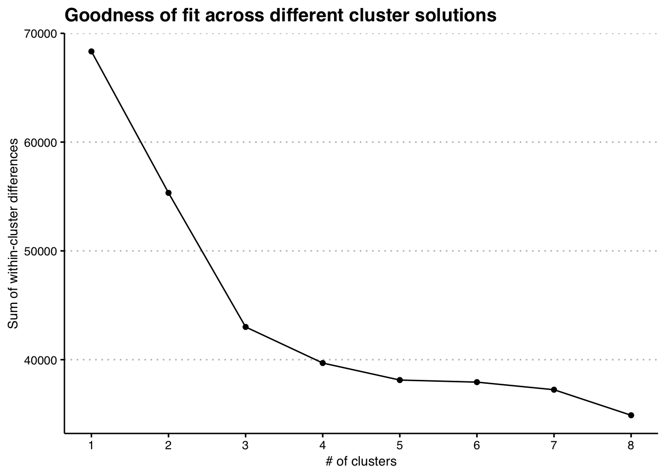
Based on the elbow plot, it appears that 3 clusters is our optimal solution, with 4 also being a possibilty. Let’s go ahead with the 3-cluster solution. What do these clusters look like? The output from fit_models() contains two tables to analyze the profile of each cluster.
Assessing clusters
The first table identifies the modal category for each variable within each cluster. It also dispalys the relative proportions of each cluster. To view this table, we simply print the table for the 3-cluster solution within our models_fit tibble.
pluck(models_fit, "table_cluster_modes", 3) # priting the table_cluster_modes column in the 3rd row| Cluster modes | |||
|---|---|---|---|
| Attributes | Cluster 1 (33%) | Cluster 2 (45%) | Cluster 3 (22%) |
| Contract | |||
| Month-to-month | |||
| One year | |||
| Two year | |||
| Dependents | |||
| No | |||
| Yes | |||
| DeviceProtection | |||
| No | |||
| Yes | |||
| No internet service | |||
| gender | |||
| Female | |||
| Male | |||
| InternetService | |||
| DSL | |||
| Fiber optic | |||
| No | |||
| MonthlyCharges | |||
| 1 | |||
| 2 | |||
| 3 | |||
| 4 | |||
| MultipleLines | |||
| No | |||
| Yes | |||
| No phone service | |||
| OnlineBackup | |||
| No | |||
| Yes | |||
| No internet service | |||
| OnlineSecurity | |||
| No | |||
| Yes | |||
| No internet service | |||
| PaperlessBilling | |||
| No | |||
| Yes | |||
| Partner | |||
| No | |||
| Yes | |||
| PaymentMethod | |||
| Bank transfer (automatic) | |||
| Credit card (automatic) | |||
| Electronic check | |||
| Mailed check | |||
| PhoneService | |||
| No | |||
| Yes | |||
| SeniorCitizen | |||
| No | |||
| Yes | |||
| StreamingMovies | |||
| No | |||
| Yes | |||
| No internet service | |||
| StreamingTV | |||
| No | |||
| Yes | |||
| No internet service | |||
| TechSupport | |||
| No | |||
| Yes | |||
| No internet service | |||
| tenure | |||
| 1 | |||
| 2 | |||
| 3 | |||
| 4 | |||
| TotalCharges | |||
| 1 | |||
| 2 | |||
| 3 | |||
| 4 | |||
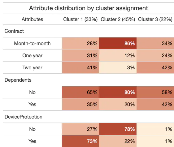
Another way of viewing the make-up of each cluster is by looking at the distribution of attribute levels within each cluster. These distributions are displayed by a heat map in the table_attribute_distribution column.
pluck(models_fit, "table_attribute_distribution", 3)| Attribute distribution by cluster assignment | |||
|---|---|---|---|
| Attributes | Cluster 1 (33%) | Cluster 2 (45%) | Cluster 3 (22%) |
| Contract | |||
| Month-to-month | 28% | 86% | 34% |
| One year | 31% | 12% | 24% |
| Two year | 41% | 3% | 42% |
| Dependents | |||
| No | 65% | 80% | 58% |
| Yes | 35% | 20% | 42% |
| DeviceProtection | |||
| No | 27% | 78% | 1% |
| Yes | 73% | 22% | 1% |
| No internet service | NA | NA | 98% |
| gender | |||
| Female | 44% | 54% | 49% |
| Male | 56% | 46% | 51% |
| InternetService | |||
| DSL | 38% | 48% | 2% |
| Fiber optic | 62% | 52% | NA |
| No | NA | NA | 98% |
| MonthlyCharges | |||
| 1 | 0% | 7% | 99% |
| 2 | 15% | 44% | 1% |
| 3 | 25% | 38% | 0% |
| 4 | 60% | 11% | NA |
| MultipleLines | |||
| No | 22% | 54% | 77% |
| Yes | 70% | 32% | 22% |
| No phone service | 9% | 14% | 1% |
| OnlineBackup | |||
| No | 32% | 74% | 1% |
| Yes | 68% | 26% | 1% |
| No internet service | NA | NA | 98% |
| OnlineSecurity | |||
| No | 44% | 78% | 0% |
| Yes | 56% | 22% | 1% |
| No internet service | NA | NA | 98% |
| PaperlessBilling | |||
| No | 32% | 32% | 71% |
| Yes | 68% | 68% | 29% |
| Partner | |||
| No | 28% | 69% | 52% |
| Yes | 72% | 31% | 48% |
| PaymentMethod | |||
| Bank transfer (automatic) | 30% | 16% | 22% |
| Credit card (automatic) | 30% | 16% | 22% |
| Electronic check | 32% | 48% | 8% |
| Mailed check | 9% | 20% | 49% |
| PhoneService | |||
| No | 9% | 14% | 1% |
| Yes | 91% | 86% | 99% |
| SeniorCitizen | |||
| No | 80% | 80% | 97% |
| Yes | 20% | 20% | 3% |
| StreamingMovies | |||
| No | 22% | 72% | 1% |
| Yes | 78% | 28% | 1% |
| No internet service | NA | NA | 98% |
| StreamingTV | |||
| No | 23% | 72% | 1% |
| Yes | 77% | 28% | 1% |
| No internet service | NA | NA | 98% |
| TechSupport | |||
| No | 41% | 80% | 1% |
| Yes | 59% | 20% | 1% |
| No internet service | NA | NA | 98% |
| tenure | |||
| 1 | 2% | 42% | 26% |
| 2 | 12% | 33% | 28% |
| 3 | 32% | 21% | 24% |
| 4 | 55% | 4% | 22% |
| TotalCharges | |||
| 1 | 0% | 35% | 42% |
| 2 | 5% | 30% | 45% |
| 3 | 25% | 31% | 13% |
| 4 | 69% | 4% | NA |
Looking through these two tables, there does appear to be clear variation across clusters, which means that our clustering model did a good job of identifying latent groups within the data. Are these groups predictive of churn?
Using clusters to predict distal outcome
To assess the relationship between cluster membership and churn, we must merge the church variable in with our data that contains cluster assignment. To get the latter, we can simply access the df column, which contains all columns used in our model, as well as cluster assignment. I’ll save this data as “clusters”.
clusters <-
models_fit %>%
  pluck("df", 3)
Because row ordering was retained, we can add the churn variable to clusters from the data_r tibble with mutate().
clusters_r <-
  clusters %>%
  mutate(churn = data_r$Churn)

glimpse(clusters_r)
## Rows: 7,032
## Columns: 21
## $ cluster <fct> 2, 2, 2, 2, 2, 2, 2, 2, 1, 2, 2, 3, 1, 1, 1, 1, 3, 1,…
## $ gender <fct> Female, Male, Male, Male, Female, Female, Male, Femal…
## $ SeniorCitizen <fct> No, No, No, No, No, No, No, No, No, No, No, No, No, N…
## $ Partner <fct> Yes, No, No, No, No, No, No, No, Yes, No, Yes, No, Ye…
## $ Dependents <fct> No, No, No, No, No, No, Yes, No, No, Yes, Yes, No, No…
## $ tenure <fct> 1, 3, 1, 3, 1, 1, 2, 2, 2, 4, 2, 2, 4, 3, 2, 4, 3, 4,…
## $ PhoneService <fct> No, Yes, Yes, No, Yes, Yes, Yes, No, Yes, Yes, Yes, Y…
## $ MultipleLines <fct> No phone service, No, No, No phone service, No, Yes, …
## $ InternetService <fct> DSL, DSL, DSL, DSL, Fiber optic, Fiber optic, Fiber o…
## $ OnlineSecurity <fct> No, Yes, Yes, Yes, No, No, No, Yes, No, Yes, Yes, No …
## $ OnlineBackup <fct> Yes, No, Yes, No, No, No, Yes, No, No, Yes, No, No in…
## $ DeviceProtection <fct> No, Yes, No, Yes, No, Yes, No, No, Yes, No, No, No in…
## $ TechSupport <fct> No, No, No, Yes, No, No, No, No, Yes, No, No, No inte…
## $ StreamingTV <fct> No, No, No, No, No, Yes, Yes, No, Yes, No, No, No int…
## $ StreamingMovies <fct> No, No, No, No, No, Yes, No, No, Yes, No, No, No inte…
## $ Contract <fct> Month-to-month, One year, Month-to-month, One year, M…
## $ PaperlessBilling <fct> Yes, No, Yes, No, Yes, Yes, Yes, No, Yes, No, Yes, No…
## $ PaymentMethod <fct> Electronic check, Mailed check, Mailed check, Bank tr…
## $ MonthlyCharges <fct> 1, 2, 2, 2, 3, 4, 3, 1, 4, 2, 2, 1, 4, 4, 4, 4, 1, 4,…
## $ TotalCharges <fct> 1, 3, 1, 3, 1, 2, 3, 1, 3, 3, 2, 1, 4, 4, 3, 4, 2, 4,…
## $ churn <chr> "No", "No", "Yes", "No", "Yes", "Yes", "No", "No", "Y…Now we will test if there are differences between groups in churn using logistic regression.
library(marginaleffects)

logit_fit <-
clusters_r %>%
  mutate(churn = if_else(churn == "Yes", 1, 0)) %>%
  glm(churn ~ cluster,
      data = .,
      family = "binomial")

ame_plot <-
logit_fit %>%
  marginaleffects::marginaleffects() %>%
  summary() %>%
  ggplot(aes(x = contrast, y = estimate)) +
  geom_pointrange(aes(ymin = conf.low, ymax = conf.high)) +
  coord_flip() +
  geom_hline(yintercept = 0,
             linetype = "dotted") +
  labs(
    x = "Average Marginal Effect",
    y = "Cluster contrasts",
    title = str_wrap("Average Marginal Effects of Cluster Membership on Customer Churn", width = 40)
  ) +
  theme_classic()

pr_plot <-
logit_fit %>%
  marginaleffects::marginalmeans() %>%
  summary() %>%
  ggplot(aes(x = value, y = estimate)) +
  geom_pointrange(aes(ymin = conf.low, ymax = conf.high)) +
  labs(
    x = "Pr(Churn)",
    y = "Cluster assignment",
    title = str_wrap("Probability of Churn by Cluster Assignment", width = 40)) +
  theme_classic()


library(patchwork)

pr_plot + ame_plot 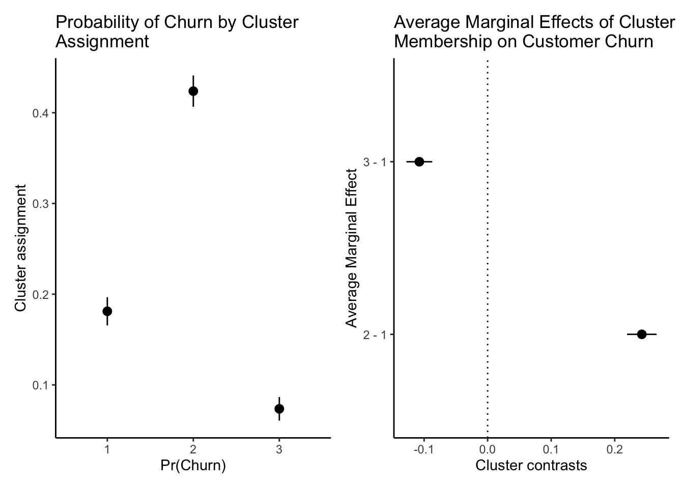
Cluster membership appears to be a strong predictor of churn, indicating that our clustering model is identifying meaningful sub-groups among customers. The telecom company could use this information to direct targeted efforts to prevent future customer churn.
Sean Bock
Research Scientist | Demography and Survey Science
I am interested in Quantitative Research, Natural Language Processing, Survey Research, and Data Visualization